Numerical Modeling Methods in Water Management
A model is a simplified representation of a true but unknown system. In water management, hydrogeologic models are developed to represent groundwater flow regimes. Hydrogeologic models are used to explain a phenomena or to predict the outcome of certain processes of an aquifer by solving the governing mathematical equations. The solution can be approached analytically and/or numerically depending on various factors such as the modeling problem itself, size and scale of the area of interest, the condition of the water system, and the availability of the data. This blog presents the advantages of the numerical approach and discusses the two most common methods for numerical modelling in hydrogeology, the finite-difference (FDM) and finite-element (FEM) methods.
Numerical models can be used to confirm the analytical solution, but much more, it’s used to handle very complex hydrogeologic systems where an analytical approach has limiting capabilities. Numerical solutions use a systematic numerical method to approximate the governing mathematical functions and, therefore, require greater initial information. Often a site characterization might be necessary to obtain reliable data. While FDM and FEM models are two common methods for numerical modeling, other methods are the finite volume method, spectral method, analytical elements, and discrete element method, which are not commonly used in groundwater applications and will not be discussed here.
The fundamental principle of the FDM and FEM models is very similar. Both approaches consider a partition of a continuous domain into numerous smaller parts (into discrete domain) where mathematical functions are calculated for each part. The differences between FDM and FEM models are in the model geometries (Figure 1) and the approach to solve the mathematical functions.

Figure 1: Finite Element model (a) and finite difference model (b) of a sphere (Hun et al., 2011)
Finite-Difference Method
The finite-difference model consists of a model “grid” that is partitioned into rectangular (2D) or cuboid (3D) pieces called “cells”. Each cell can be further discretized, which means, parted into smaller cells, to obtain higher resolution of the model to get a better accuracy of the calculation if sufficient data are available to warrant the higher resolution. The refinement of the grid occurs vertically and/or horizontally of the area of interest. Figure 2 (below) shows how a real-world situation is conceptualized in the model (“Conceptual Model”), and how the river and well are represented in a FDM model (“Finite Difference Grid”), with greater resolution near the well. Due to the shape of the cell (i.e., rectangular or square), the FDM model domain often expands beyond the model area. However, these areas outside the principal area of interest in the model can be assigned as “inactive” cells to eliminate unnecessary cells. The model calculates the governing differential equation by approximating the derivatives of the finite difference equation for each cell. In other words, consider a point in space where an infinite equation is replaced by sections of the equation – the finite difference equation. This solving approach works well with regular rectangular or square-shaped elements and requires less computational effort.
MODFLOW is a popular modular FDM modeling software developed by the USGS for flow simulation of surface water and groundwater.
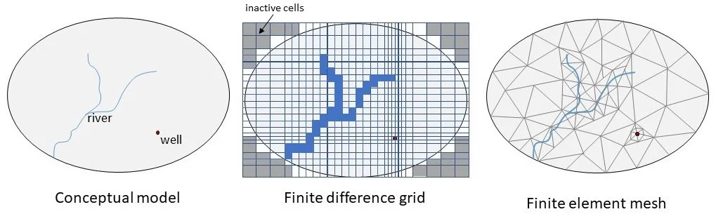
Figure 2: Model Domain of Finite Difference and Finite Element Models
Finite-Element Method
The finite element model consists of a “mesh” with irregular triangular (2D) or quadrilateral (3D) elements. An element in a mesh of a finite element model can be compared to a cell in a grid of a finite difference model. Different than a FDM model, calculations are carried out on the nodes, which are the vertices of each element. Due to the flexibility of a mesh, the model can represent the exact geometry of an irregular model shape. Furthermore, the discretization can be refined locally, around the area of interest.
Figure 2 (above right) depicts a mesh refinement for the same river and well as depicted in a FDM model, and the river as simulated in a FEM model. FEM models formulate the partial differential equation for each node and the results are then put together into one solution that is reasonable for the entire domain. This approach can achieve higher accuracy in exchange for higher computational effort. Hydrogeologists use FEM based program e.g. FEFLOW or HYDRUS, for the simulation of groundwater flow, as well as heat and mass transport in porous media.
FEM models are preferred where model geometry is of importance such as the modelling of the aerodynamics of a plane, F1 racing car, or a space shuttle. For surface water and groundwater modeling both FDM and FEM are suitable. The accuracy of model results does not only depend on the solution method, but more on the ability to translate the problem into a conceptualized model and model development, proper discretization, accuracy of the input parameter, and the calibration quality.
LWS has an experienced team of modelers that routinely use numerical models to evaluate complex surface water and groundwater hydrology issues, as well as address fate and transport of contaminants in groundwater. In addition, LWS often teams with other professionals to provide additional services related to modeling (click here for more information on collaborative modeling projects). For more information, please contact LWS at 303-350-4090 or contact our modeling team.
Anna Elgqvist, Senior Engineer, anna@lytlewater.com
Bruce Lytle, President, LWS, bruce@lytlewater.com
Subscribe to LWS Blogs HERE!
References:
Maliva R., Missimer T. (2012) Groundwater Flow and Solute-Transport Modeling. In: Arid Lands Water Evaluation and Management. Environmental Science and Engineering (Environmental Engineering). Springer, Berlin, Heidelberg
Diersch HJ.G. (2014) Fundamental Concepts of Finite Element Method (FEM). In: FEFLOW. Springer, Berlin, Heidelberg
Frey, P. (2008) Chapter 6 The finite difference method. Numerical simulation of complex PDE Problem Part II: Numerical Methods. Elective course and advanced seminar of mathematics. University of Chile. (etrieved March 11, 2020 from https://www.ljll.math.upmc.fr/frey/cours/UdC/ma691/ma691_ch6.pdf
Frey, P. (2008) Chapter 7 The finite element method. Numerical simulation of complex PDE Problem Part II: Numerical Methods. Elective course and advanced seminar of mathematics. University of Chile. Retrieved March 11, 2020) https://www.ljll.math.upmc.fr/frey/cours/UdC/ma691/ma691_ch7.pdf
Hun, J. , Chung, M. , Park, M. , Woo, S. , Zhang, X. , Marie, A. , 2011. Generation of realistic particle structures and simulations of internal stress: A numerical/AFM study of LiMn 2 O4 particles. J. Electrochem. Soc. 158, A434–A442 .
Sjodin, B. (2016) What’s the difference between FEM, FDM, and FVM? Retrieved 3/11/2020 from https://www.machinedesign.com/3d-printing-cad/fea-and-simulation/article/21832072/whats-the-difference-between-fem-fdm-and-fvm
Wexler, E.J. (2013) Transient Modelling of Groundwater Flow, Application to Tunnel Dewatering. Retrieved March 12, 2020 from https://www.slideshare.net/DirkKassenaarMScPEng/transient-modelling-of-groundwater-flow-application-to-tunnel-dewatering.